Recently a new reader emailed me, asking for an Excel (or OpenOffice) spreadsheet that could tell him what payment would be required in order to retire a loan within a certain time period. I figure I can help him out and present a very basic Excel tutorial, all in one shot. So here goes!

Calculating a Payment in Excel

Excel just so happens to have a function to calculate the payment of any loan that has (1) a constant payment, and (2) a constant interest rate. This blessed function is called PMT.

In Excel, function PMT returns a loan's payment (principal and interest) and looks like so:

=PMT(Rate,Nper,Pv,Fv,Type)

1. Rate: The interest rate of the loan;


2. Nper: The number of periods (or payments) of the loan;


3. Pv: The present value (or principal, or current balance) of the loan;


4. Fv: The future value, or balance you'll have when the last payment is made;


5. Type: Designated by either 1 or 0 (zero). Tells Excel whether payments are made at the beginning (1) or end (0 or blank) of the period.

Actually, in our example, function PMT requires only three of these inputs. You can leave "Fv" and "Type" blank; Excel will assume both to be zero.

So let's say we've been good patriotic customers of GWB National Bank (a purely fictional entity, of course). We have a loan with them which shows a current balance of $5,800. That's our loan's "present value," which means it's the "Pv" in the PMT function. GWB Nat'l Bank charges us an annual interest rate 16.99 percent; this (with a tweak) becomes the "Rate" in the PMT function. But we're on a debt-paydown kick, and now we'd sure like to have this loan paid off in 14 months (the "Nper"). Exactly what payment would be required to get this done?

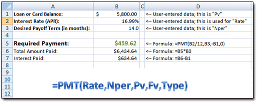
Here's how I set things up in Excel:



Cells B1, B2, and B3 contain our data above — the Pv, the Rate, and the Nper, respectively.

Cell B5 is where the PMT function resides. Remember that the function is:

=PMT(Rate,Nper,Pv,Fv,Type)

... so in our spreadsheet, the function should be:

=PMT(B2/12,B3,-B1,0)

Watch Rate and Nper!

Astute readers will note that the PMT function doesn't simply refer to our "Rate" of 16.99% (Cell B2). Rather, to get "Rate," we must divide Cell B2 by 12. Why's this? Well, since we're interested in a loan term that denoted in months, and since our loan uses monthly payments, we have to convert the APR (that's Annual Percentage Rate) in Cell B2 to an equivalent monthly periodic rate. So we divide Cell B2 by 12. That gives us the monthly periodic rate. Now the relevant variables — Rate and Nper — are on a "monthly" basis, and Excel's PMT function can do its thing correctly.

All Worked Out

As we can see in Cell B5, a payment of $459.62 would be required to retire our loan in fourteen months. Just for kicks 'n' giggles, we can also have Excel show us how much we'll pay (in total) during those fourteen months. That's what you see in Cell B6, where the formula simply multiplies our monthly payment (B5) by the loan term (B3).

From there, it's a snap to see how much interest we'll pay during the term. In Cell B7, I simply take the total amount paid (B6) and from it subtract the starting balance (B1). The difference between those two figures is all interest, baby.

Get the Spreadsheet

You can get the spreadsheet shown above by downloading it here.

Labels: Debt, Excel