The requirement that puzzled her? She had to use Excel's SUMIF function somewhere in her check-register spreadsheet.
After a few minutes of thought, I suggested that she add a column for Transaction Type (CKCD, CASH, CHK, DEP) if she hadn't done so already. She could then use the SUMIF formula in a cell somewhere to total up, say, all the deposits (type DEP) in the register. "Could be useful to someone," I wrote.
That was also approximately when I thought to myself: Hey! Why not do a how-to blog post for the SUMIF function?
So, those of you who are bored to tears by my Excel how-to posts can stop here and go do something exciting, like grabbing a rubber-band gun and thwapping the politicians on CSPAN. They deserve it; trust me.
Using Excel's SUMIF Function
Most folks know that in Excel, the SUM function is used to add up (sum) a group of numbers. The SUMIF function goes beyond that: It sums a group of numbers, yes, but it sums only those numbers which fit some user-designated criteria.
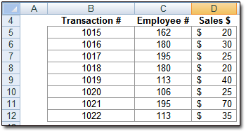
For instance, consider the following chart:

We could execute the SUM formula on Column D, the Sales column, like so:
This would give us the total sales amount for all transactions. However, what if we simply want to know how much employee 180 sold? That's where the SUMIF function comes in!
The SUMIF function has three arguments...

... where:
- "Criteria_range" is the range of cells which contain the criteria we're searching through;
- "Criteria" is the specific criteria/condition we wish to match; and
- "Sum_range" is the range of cells in which selected numbers will be summed.
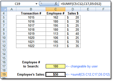
So, in our case above, we wish to sum up the sales of employee 180. We'll put our SUMIF function in Cell C19. A finished version might look like so:

Our "criteria_range" is C5:C12 (the range of employee numbers). Our "criteria" is Cell C17, where we've input the employee number whose total sales we wish to calculate. And our "sum_range" is D5:D12, the range of sales figures.
With this info plugged into our SUMIF function in Cell C19, Excel tells us that employee 180 booked $50 of revenue. (And some quick gradeschool math tells us Excel is correct!)
For those of you who'd like to view it, my SUMIF Example Spreadsheet (.xls) can be downloaded as a ZIP file and extracted.


